The bear market logic for gold miners: Continuation and Analysis

The summer slump for precious metals has turned into a nightmare, with gold breaking below $1100, platinum into the triple digits and silver well below $15. While the July slide is pretty bad, what makes it worse is precious metals setting fresh multi-year lows.
Compared to the plunge among miners however, the precious metals sell-off seems rather meek: the HUI/Gold ratio is threatening to drop below 0.100, which is five times lower than its 2003-08 equilibrium level and over four times lower than where HUI/Gold recovered to in 2009-2010. In May, I drafted an article titled: Gold and the miners: identifying the bear market logic. After the latest sell-off it is worth checking whether the bear-market-logic for the miners still holds.

Identifying the bear market logic

Let's start with an update of the graph the previous article ended with: Gold price (left scale) and the HUI miners index (right scale) are shown to match rather well. The oscillatory down trend of the HUI/Gold ratio ever since 2011 implies that a proportional logic is not holding any longer.

Gold (red, left scale in USD/Oz) and HUI (blue, right scale); Data till Dec 31, 2015 - click to enlarge

The time scale extends from July 2013, as gold started recovering after its major slide since April 2013 till the present day. There still is a match of about 25 points on the HUI index to a $50 variation on the gold price. One very important difference though: the 'zero level' on the HUI would match to a reading of $850/Oz for gold. The fresh rule then is approximated by: HUI = 0.5 * (Gold price - $850)

This essentially makes the relationship non-proportional and implicitly assumes that a gold price of $850/oz would imply the gold miners to go out of business. A disclaimer not without any reason: there is no such clear 'cut-off' gold price for the mining industry. The level of the USD-index highly affects mining costs for the majority of gold producers outside the US. Moreover, gold producers have vastly different margins and most probably also high margin differences among their individual gold mining sites. Yet a rule with only two parameters is most elegant ... while the bear market logic holds.

Least squares regression

The above equation was derived graphically and parameters were rounded to make major divisions on the left (Gold) and right (HUI) axis coincide. A (least square) regression analysis provides you with mathematically exact values. Yet, even though we didn't yet implement the correct parameters obtained from a linear least squares regression, we already notice that the latest slide of gold is matched well by the continued plunge of the miners.

For a least squares linear regression, we opt to extend the interval of the gold slide from about $1800 to the latest $1090 on July 23. We then need to include data going back to September 2012, when gold failed its last attempt to break above $1800. Any time interval chosen necessarily yields a slightly different set of parameters, however including these earlier data even improves the correlation coefficient to 0.968. This corroborates the analysis results.

 May 2012 to July 2013: Gold - HUI spread (blue dots) and regression trend line (red). (click to enlarge)
September 2011 to April 2012 (Gold, HUI) values are shown in orange.

In a regression analysis, dates are eliminated: it shows the HUI values relative to the gold price. All blue dots are given (HUI, Gold) couples for any given date between Aug 1, 2012 and Dec 31, 2015.
Note: The regression made is y-values: Gold price on x-values : Hui index. It provides the intercept on the gold price axis and the inverse value of the slope of HUI relative to gold.

Using these data, the slope and intercept are 0.555 and $893, turning the HUI dependency on gold into

HUI = 0.555 * (Gold Price - $ 893) 

Including earlier (2012) data, the slope steepens, while the intercept value increases. Why we don't include data going back to September 2011 also is obvious. Those data couples are shown in orange. When checking carefully (clicking the graph for full resolution), those data points are in a cloud at the upper right, systematically above the points after Aug 2012. Including those data tilts the regression line even higher, but it deteriorates the correlation coefficient. During 2011 - when the HUI failed to catch up with the gold price steaming up to its August/September all time high - the HUI/Gold relationship was undergoing its major paradigm shift. The 'bear-market logic' only set in after gold made a few more failed attempts to break and hold above $1800.

Analysis of the residuals

While the trend line gives an overall decent fit, data points in the intermediate area seem to concentrate on the downside, while the data cloud at the right is quite extended. In the $1200-$1300 area, you find more points above the trend line than beneath. For a meaningful explanation, we need to introduce the dates once again, showing the 'residuals' as a function of time. These distances from the least squares trend graph are shown as a function of time on the below graph:

Residuals as a function of time from May 2012 till Dec 31, 2015 (click to enlarge)

Residuals are oscillating around the trend line. In 2012-13 the amplitude of the oscillations used to be quite large, giving rise to the more extended data cloud preponderant at higher gold prices. Their amplitude is reducing in 2014-2015. The data cloud now is more narrow. Both on May 29 (when the last update to previous article was made) and on July 23, the residual is positive but very close to zero. It has dropped negative during June till mid July. A negative reading implies that mining investors on average accept selling their mining shares at lower prices than what the 'bear market rule' suggests. At any positive reading, investors are ready to pay more. The sign and trend of the residuals is not meaningless at all. A negative reading sometimes is the prelude for a slide of the gold price. Strongly positive residuals may anticipate a trend reversal or corroborate any nascent gold recovery.

A 'textbook example' is shown in the graph below, where the residuals are plotted together with the gold price before and after the hectic gold sell-off in April 2013 continuing to June 2013.

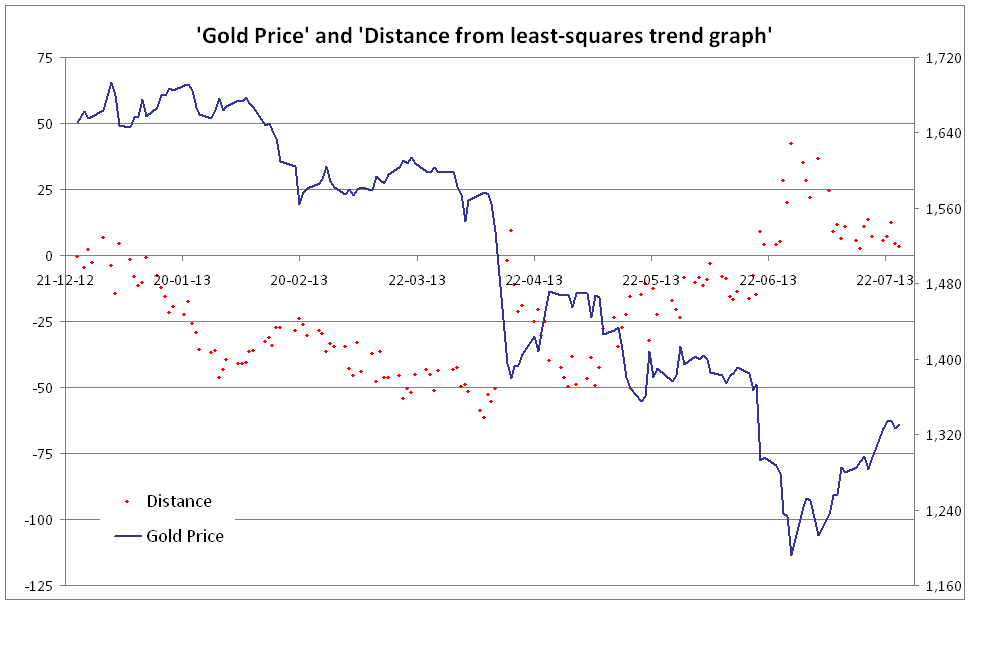Residuals (red dots, left scale) as a function of time from Christmas eve 2012 till July 26, 2013,
The gold price in USD (blue graph) is shown on the right scale. (click to enlarge)

As we head into 2013, the residuals turn negative, reaching an extreme over -50 in April, with gold near its $1560 support, shortly before the gold sell-off. It seems as though mining investors were 'sensing' what was going to happen. After the slide materialized, the residuals very briefly turned positive, yet they slid down again at the gold recovery above $1450. As gold sold off again in June, bottoming below $1200 for the first time since 2010, residuals turn up and become strongly positive. Did mining investors anticipate that these prices would not hold in the short run and that some recovery was looming? Apparently so.

And of course: since the model could be established and its parameters correctly estimated only long after the April 2013 gold price sell-off, any mining investor perception on potential gold price trend was purely intuitive. The negative reading of the residuals could not have been known nor assessed.

Most recent post

• Last article on this subject: Regression between the gold price and the HUI miners index (26-04-2017)